21 Bivariate statistics
Bivariate means “involving two variables” in statistics. It’s a method used to analyze relationships between two variables, studying how their values might connect or influence each other.
One crucial element of bivariate analysis is evaluating the correlation between two variables, which can be positive (both rise together), negative (one rises while the other falls), or non-existent (no apparent connection).
Bivariate data is often visualised using scatter plots (see Section 21.1), which can help reveal patterns or trends between the two variables.
21.1 Scatter plots
Scatter plots are glorious. Of all the major chart types, they are by far the most powerful. They allow us to quickly understand relationships that would be nearly impossible to recognize in a table or a different type of chart… Michael Friendly and Daniel Denis, psychologists and historians of graphics, call the scatter plot the most “generally useful invention in the history of statistical graphics.”
Dan Kopf
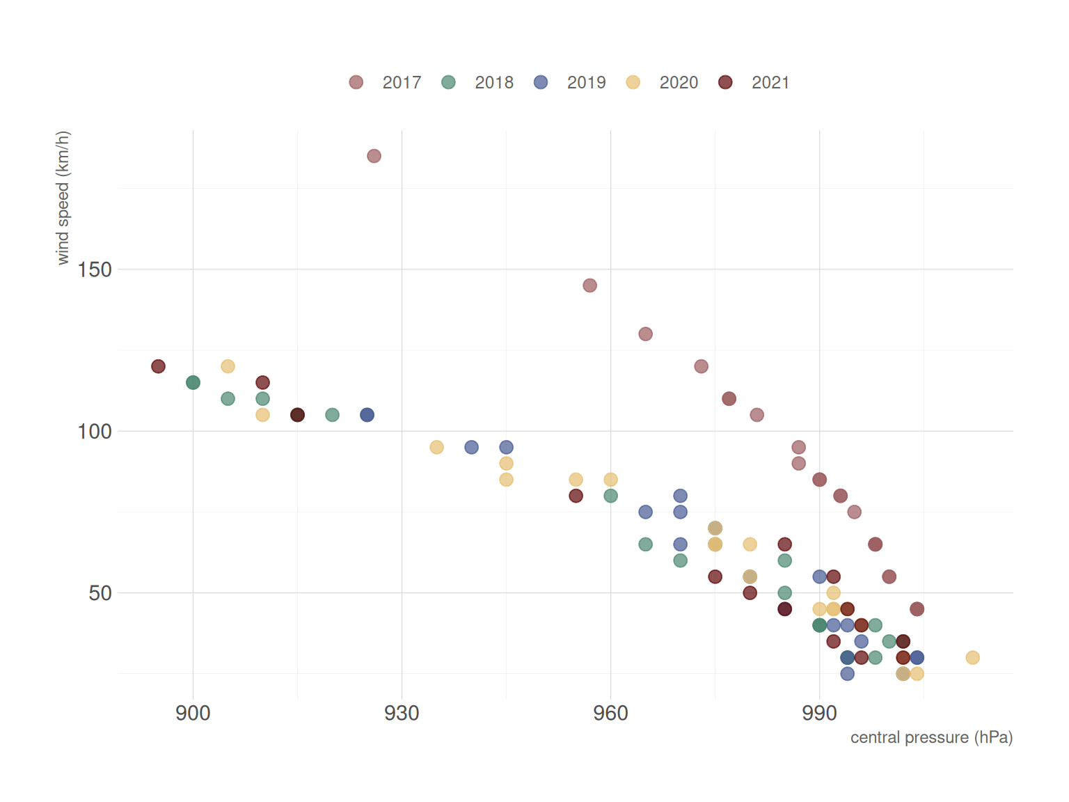
Scatter plots are graphs that show how two numerical datasets relate. Each data point is represented by a dot, positioned based on the values of the two variables being compared. They effectively demonstrate both the strength and direction of connections between these variables.
Scatter plots primarily help visualise and determine potential relationships or correlations between two variables. They reveal if the variables trend upward together (positive correlation), downward together (negative correlation), or exhibit no noticeable connection.
A scatter plot features two axes—the horizontal x-axis and vertical y-axis. Data points are represented as dots, each positioned according to their respective x and y values.
Examining the pattern of dots in a scatter plot offers insights into the relationship between variables. For example, dots forming an upward-sloping line indicate a positive correlation, whereas a downward slope suggests a negative correlation.
21.1.1 Creating scatter plots
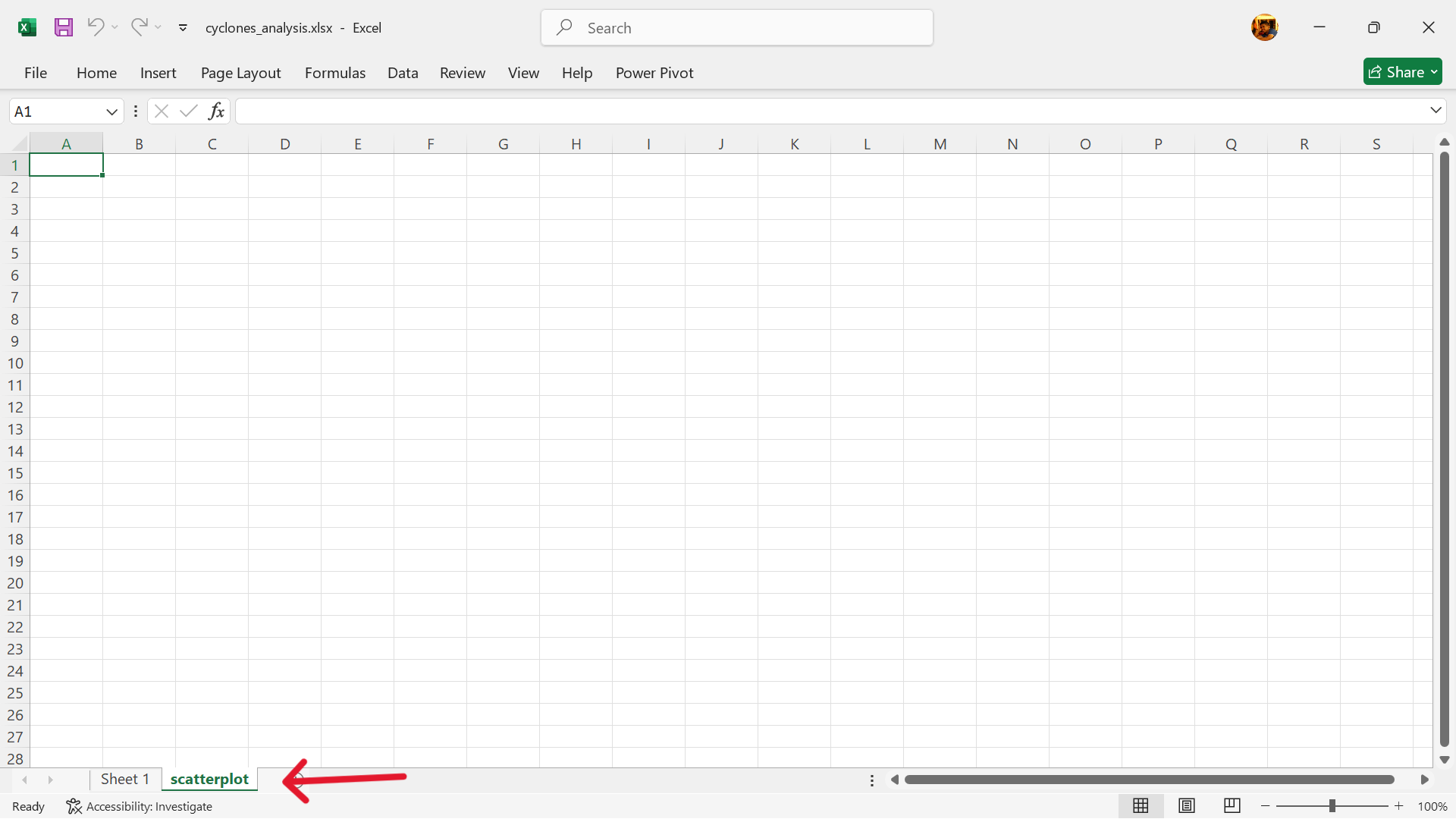
Excel has a built-in functionality to create scatterplots. Following are the steps to create a scatterplot in Excel. For this demonstration, we use the cyclones dataset. We recommend creating a new Excel workbook and import the raw cyclones dataset into this workbook to avoid contamination of the original data.
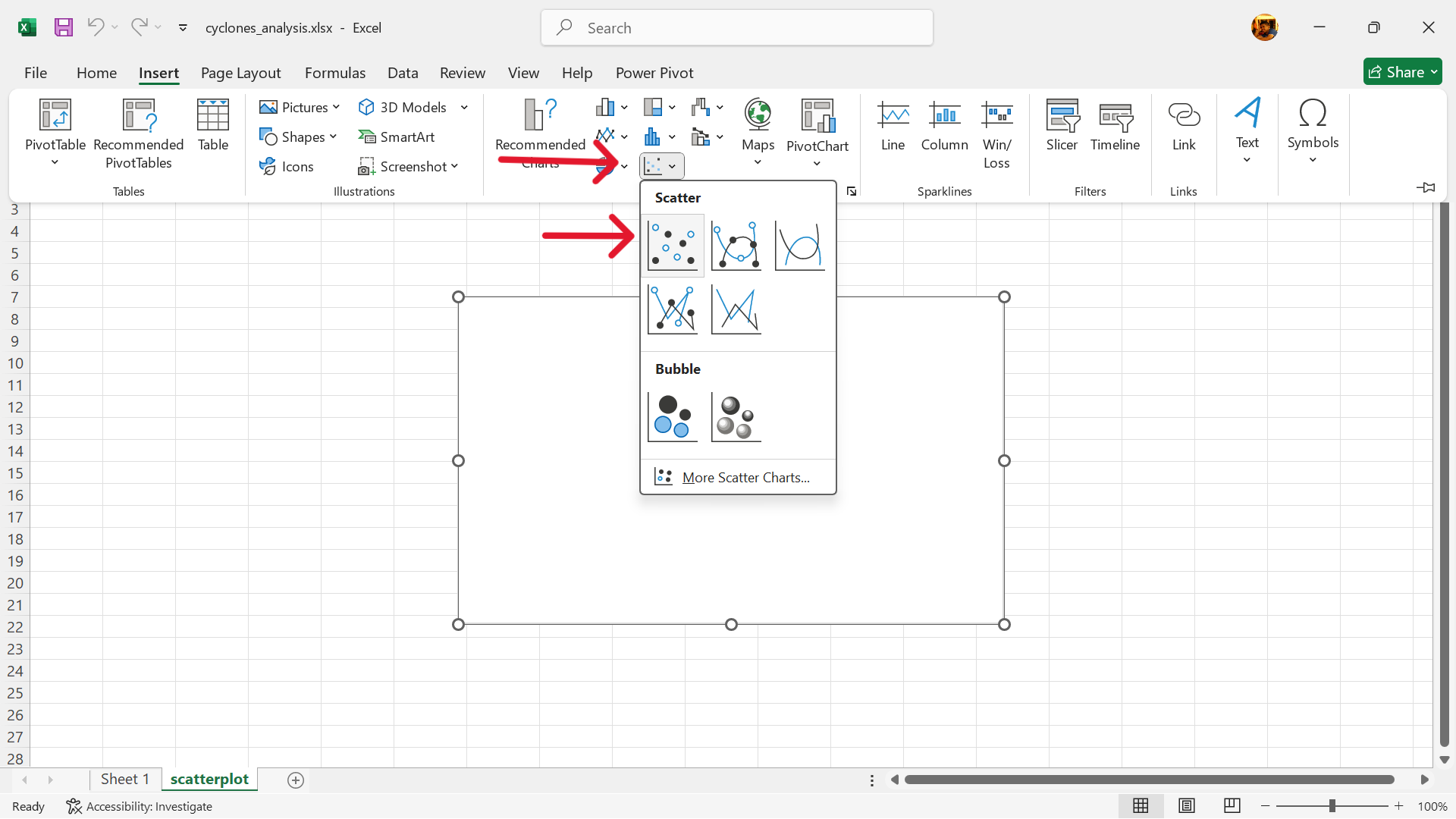
- Create a base scatterplot.
In a new worksheet, go to Insert –> Insert Scatter (X, Y) or Bubble Chart –> Scatter
- Select data to use for the scatterplot.
- Select base scatterplot –>
Chart Design–>Select Data
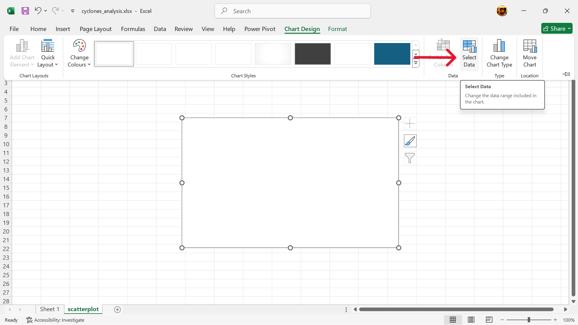
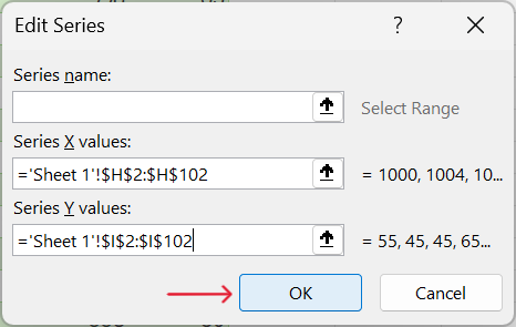
- Click on
Addto add a new data series (Figure 21.5).
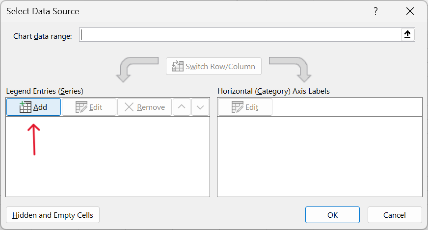
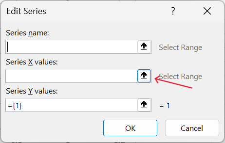
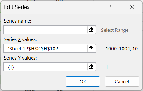
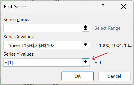
- Select the appropriate x-axis and y-axis values. For this demonstration, we will use pressure as the x-axis variable and speed as the y-axis variable.
- Add a trendline (Figure 21.10).
Chart Elements –> Trendline –> Linear
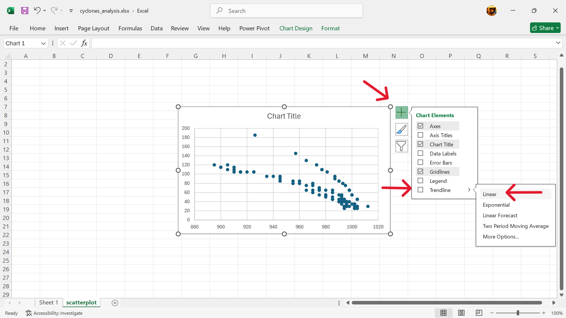
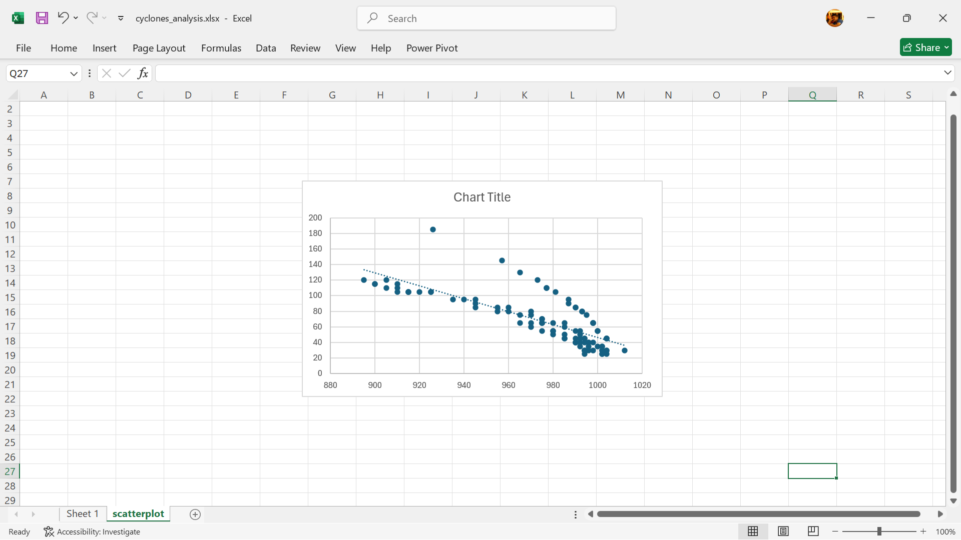
- The scatterplot is now created (Figure 21.11).
21.2 Numerical measures of association
21.2.1 Correlation
Correlation is a statistical measure indicating how strongly and in what direction two variables are connected. While it reveals the extent and nature of a linear relationship, it does not imply that one variable causes the other - it only shows how often they move together without explaining why.
21.2.2 Correlation measures
In this section, we discuss the three most common numerical measures of correlation - Pearson’s correlation coefficient, Spearman’s rank correlation coefficient, and Kendall’s tau rank correlation coefficient.
Of these three, Spearman’s and Kendall’s are non-parametric and are considered more robust than Pearson’s.
Pearson’s correlation coefficient
Pearson’s correlation coefficient, commonly referred to as Pearson’s \(\rho\), is a statistical tool used to evaluate both the strength and direction of a linear association between two continuous variables. It indicates how closely data points align with a line of best fit. The value of \(\rho\) can range from -1 to +1.
The absolute value of Pearson’s \(\rho\) reflects the strength of the linear relationship. A score of 1 or -1 signifies a perfect positive or negative correlation, respectively, implying all data points lie perfectly on a line. Conversely, a score of 0 suggests no linear relationship exists.
Pearson’s \(\rho\) can be calculated as follows:
\[ \rho ~ = ~ \frac{covariance(x_1, x_2)}{(n-1) sd_{x_1} sd_{x_2}} \]
where
\(x_1,x_2 ~ = ~ \text{continuous variables to test correlation of}\)
\(n ~ = ~ \text{number of data pairs for } x_1,x_2\)
\(sd_{x_1},sd_{x_2} ~ = ~ \text{standard deviation for } x_1,x_2\)
In Excel, either the PEARSON() or the CORREL() function is used to get Pearson’s \(\rho\). To get Pearson’s \(\rho\) for the correlation between pressure and speed from the cyclones dataset, we use the following calculation:
=PEARSON(H2:H102,I2:I102)or
=CORREL(H2:H102,I2:I102)with both giving a Pearson’s \(\rho\) of -0.7886634.
Table 21.1 summarises how to interpret the range of Pearson’s \(\rho\) values.
| Pearson’s \(\rho\) | Interpretation |
|---|---|
| +1 | Perfect positive correlation |
| -1 | Perfect negative correlation |
| 0 | No correlation |
| +/- 0.1 to +/- 0.3 | Weak correlation |
| +/- 0.4 to +/- 0.6 | Moderate correlation |
| +/- 0.7 to +/- 0.9 | Strong correlation |
It’s important to note that Pearson’s \(\rho\) only measures linear relationships. It may not accurately reflect the relationship between variables if the relationship is non-linear. Pearson’s correlation is typically used when dealing with normally distributed data that are measured on interval or ratio scales.
Spearman’s rank correlation coefficient
Spearman’s rank correlation coefficient (Spearman’s \(\rho\)) is a statistical measure that assesses the strength and direction of a monotonic relationship between two ranked variables. It’s a non-parametric test, meaning it doesn’t assume data follows a normal distribution and is often used when data is ordinal or when a linear relationship isn’t assumed. The coefficient ranges from -1 to +1, with -1 indicating a perfect negative correlation, +1 indicating a perfect positive correlation, and 0 indicating no correlation.
Compared to Pearson’s \(\rho\), Spearman’s \(\rho\) performs the correlation test on the rank of the values of the two variables rather than on the values themselves.
Hence, the values of the two variables are ranked first and then the Spearman’s \(\rho\) is calculated based on these ranks as follows:
\[ \rho ~ = ~ 1 - \frac{6 \sum d ^ 2}{n(n ^ 2 - 1)} \]
where:
\(d ~ = ~ \text{difference in ranks}\)
\(n ~ = ~ \text{number of data pairs}\)
In Excel, we can calculate Spearman’s \(\rho\) as follows (using the pressure and speed variables in the cyclones dataset):
- Rank each of the two variables you are testing for correlations using the
RANK.AVG()function.
For this step, we recommend creating a new worksheet and importing the raw dataset to this worksheet to avoid contamination of the raw data (Figure 21.12).
Create a new variable for the ranking of the pressure variable and then rank using RANK.AVG() function (Figure 21.13).
Create a new variable for the ranking of the speed variable and then rank using RANK.AVG() function (Figure 21.14).
- Calculate Spearman’s \(\rho\).
- Calculate using the
CORREL()function in Excel.
The CORREL() function should be applied to the ranks for pressure and speed (see Figure 21.17) instead of the actual pressure and speed values (as used in the Pearson’s calculation).
=CORREL(J2:J102,K2:K102)Using this method, the Spearman’s \(\rho\) for pressure and speed variable in the cyclones dataset is -0.8289627
- Calculate using the formula.
First, get the square differences of the pressure and speed ranks (Figure 21.18).
=(J2-K2)^2Then apply the Spearman’s \(\rho\) formula as follows:
=1-((6*SUM(L2:L102))/(COUNT(L2:L102)*(COUNT(L2:L102)^2-1)))Using this method, the Spearman’s \(\rho\) for pressure and speed variable in the cyclones dataset is -0.8226878
Note 21.1: Difference between built-in function result and the calculated result
There is a very small difference (-0.0063) between the result when CORREL() function is used compared to when the formula is used. This is likely due to some differences in the way ranking is performed by the CORREL() function compared to the RANK.AVG() function approach used in the calculation approach.
The reference table in Table 21.1 for the Pearson’s \(\rho\) can also be used to interpret Spearman’s \(\rho\).
Kendall’s rank correlation coefficient
Kendall’s \(\tau\), alternatively referred to as Kendall’s tau rank correlation coefficient, serves as a statistical tool for evaluating the ordinal relationship between two variables. It examines how closely the rankings of data points align across two datasets, irrespective of their specific values. This measure is non-parametric, implying it does not rely on assumptions about data distribution and remains effective even in the presence of outliers.
Kendall’s \(\tau\) assesses how closely the rankings of two variables align. If one variable’s ranking rises, does the other also tend to rise (positive relationship), fall (negative relationship), or show little pattern (nearly zero correlation)?
The method involves comparing concordant pairs - where both variables’ rankings follow the same order - and discordant pairs - where their rankings are opposite in order.
Kendall’s \(\tau\) can be calculated as follows:
\[ \tau ~ = ~ \frac{n_{concordant} - n_{discordant}}{\frac{n (n-1)}{2}}\]
where:
\(n ~ = ~ \text{number of data pairs}\)
There is no built-in function in Excel that calculates Kendall’s \(\tau\). Following are steps on how to arrive at this value for pressure and speed variables in the cyclones dataset using Excel.
- Create a new worksheet and import cyclones dataset.
We recommend creating a new worksheet and importing the raw dataset to this worksheet (see Figure 21.20) to avoid contamination of the raw data.
- Rank pressure values.
Using the RANK.AVG() function in Excel, rank the pressure values as follows (Figure 21.21):
=RANK.AVG(H2,$H$:$H$102)- Rank speed values.
Using the RANK.AVG() function in Excel, rank the speed values as follows (Figure 21.23):
=RANK.AVG(I2,$I$:$I$102)- Sort the table by ascending order based on the pressure rank.
Click on the sort functionality at the pressure column if available (Figure 21.25) or go to Data –> Sort to sort the table by pressure rank in ascending order.
- Create new variable for counts of concordant pairs.
Concordant pairs are items that are ranked higher in variable X and also ranked higher in variable Y, or items ranked lower in X and also ranked lower in Y.
Since our cyclones data is now sorted in ascending order based on the pressure ranking, we can go down the array of ranks for speed to check for concordance. For example, in the cyclones dataset, if the value of the speed rank in K2 cell is higher than the value of the rank in the K3 cell, then these two are counted as concordant pairs. We make this comparison for the speed rank in K2 for every cell after it and tally the number of concordant pairs. The sum of the counts of concordant pairs for K2 cell becomes the value for the concordant variable for row 2. We then do the same for the next row until we have counts of concordant pairs for each row of data.
This can be implemented in Excel using the following formula (Figure 21.27):
=COUNTIF(K3:$K$102,">"&K2)- Create new variable for counts of discordant pairs.
Discordant pairs are items that are ranked higher in variable X and are ranked lower in variable Y, or vice versa.
Since our cyclones data is now sorted in ascending order based on the pressure ranking, we can go down the array of ranks for speed to check for concordance. For example, in the cyclones dataset, if the value of the speed rank in K2 cell is lower than the value of the rank in the K3 cell, then these two are counted as discordant pairs. We make this comparison for the speed rank in K2 for every cell after it and tally the number of discordant pairs. The sum of the counts of discordant pairs for K2 cell becomes the value for the discordant variable for row 2. We then do the same for the next row until we have counts of discordant pairs for each row of data.
This can be implemented in Excel using the following formula (Figure 21.29):
=COUNTIF(K3:$K$102,"<"&K2)- Calculate Kendall’s \(\tau\).
Now that we have the counts of concordant and discordant pairs, we can calculate Kendall’s \(\tau\) in Excel as follows (Figure 21.31):
=(SUM(L2:L102)-SUM(M2:M102))/((COUNT(L2:L102)*(COUNT(L2:L102)-1))/2)This results in a Kendall’s \(\tau\) of -0.642178218.
The reference table in Table 21.1 for the Pearson’s \(\rho\) can also be used to interpret Kendall’s \(\tau\).