22 Epidemiological statistics
In this chapter, we will cover topics and techniques on statistical methods commonly used by epidemiologists in public health investigations or studies that have wider uses and applications to other fields. These methods are considered bread-and-butter techniques for all epidemiologists and are generally easy to implement.
We will cover topics on contingency tables, relative risk ratio, odds ratio, and t-test. These methods can be considered bivariate statistics as they are applied on two variables but with binary categorical variables. To demonstrate these techniques, we will use the fem dataset.
22.1 Contingency tables
A contingency table, also known as a cross-tabulation, is used in statistics to display the relationship between two or more categorical variables. It organises data by showing the frequency of observations that fall into various combinations of the categories of the variables being examined. It is also usually called a two-by-two table as its common use is for comparing two categories per group. However, contingency tables can also be created with more than two categories per group.
For this topic, we will focus on two-by-two tables for simplicity and to be consistent with exploratory data analysis of bivariates.
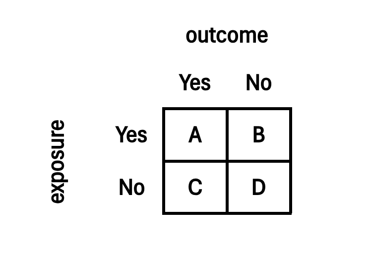
Figure 22.1 demonstrates the structure of a two-by-two contingency table with the exposure variable on the rows and the outcome variable on the columns.
Since contingency tables were developed for disease epidemiology, the term exposure has been used which usually pertains to exposure to a risk factor or known causative agent of a particular disease outcome.
However, exposure in a general sense can also mean exposure to a factor or a condition that is known to be associated to a certain outcome which doesn’t have to be a disease. For example, exposure to being female for an outcome of good grades; exposure to being married for an outcome of owning your house, etc.
22.1.1 Creating two-by-two contingency tables
In Excel, a contingency table can be easily created using pivot tables. Using the fem dataset, we can create a contingency table for the exposure variable of lost interest in sex (SEX variable) and the outcome variable of considered suicide (LIFE variable) through the following steps.
- Create a new worksheet for the contingency table.
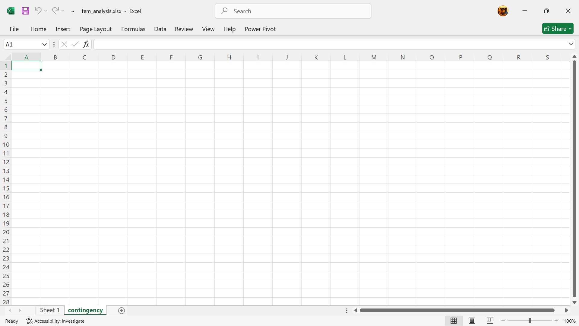
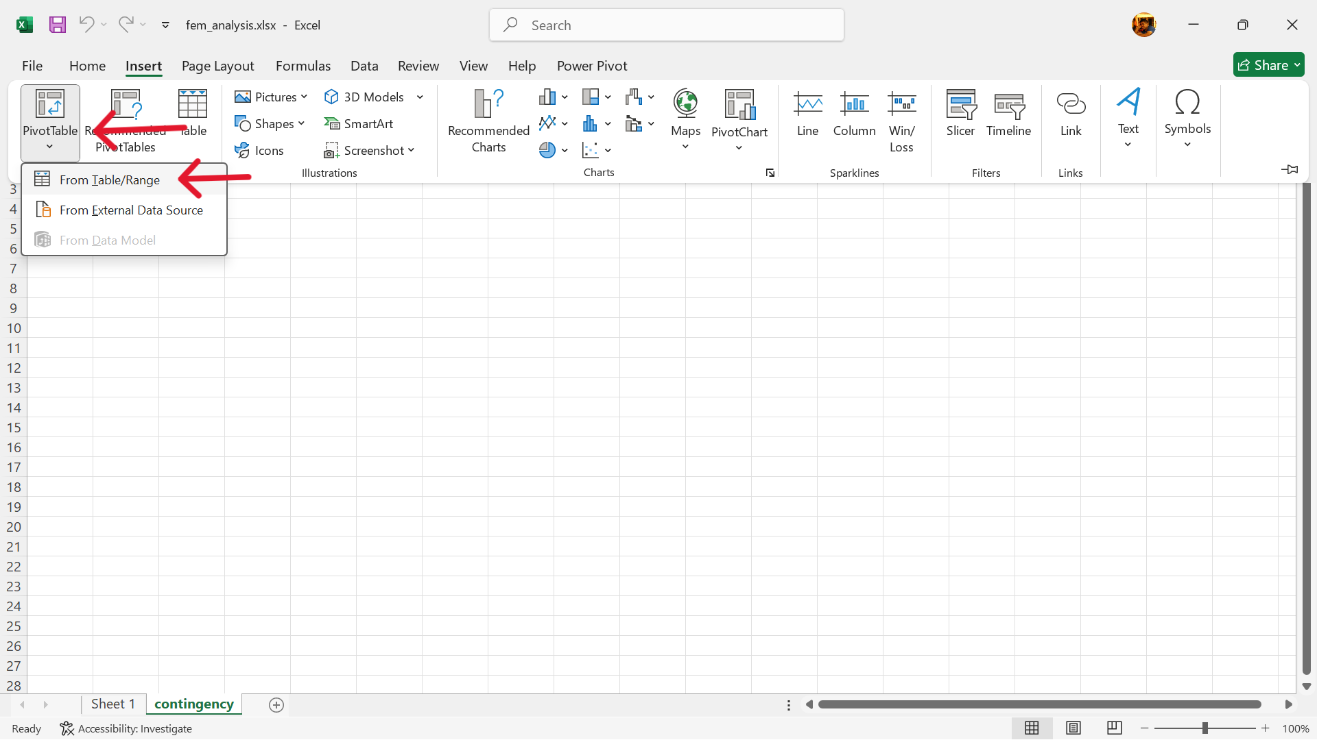
- Setup pivot table.
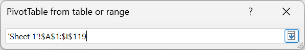
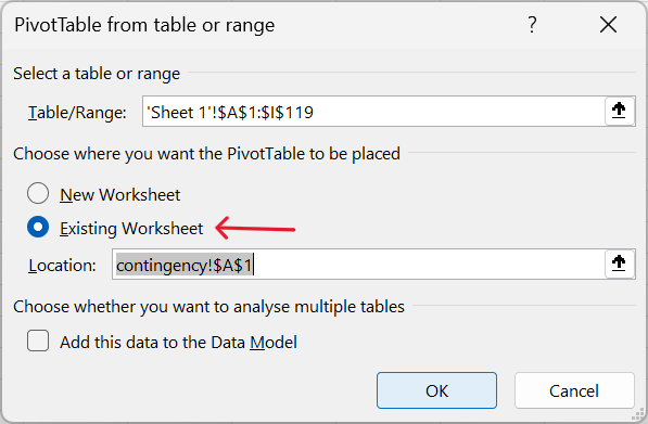
Insert–>Pivot Table–>From table/range
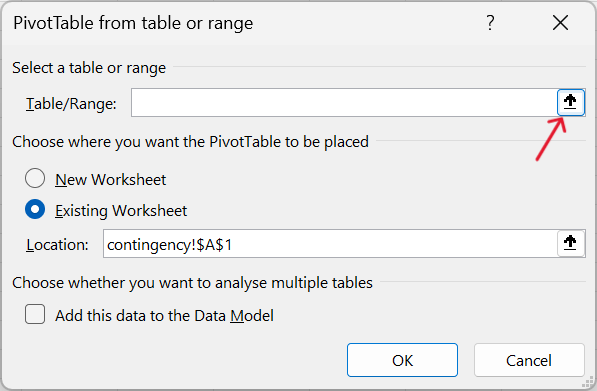
- Select table/range to pivot and insert into current worksheet.
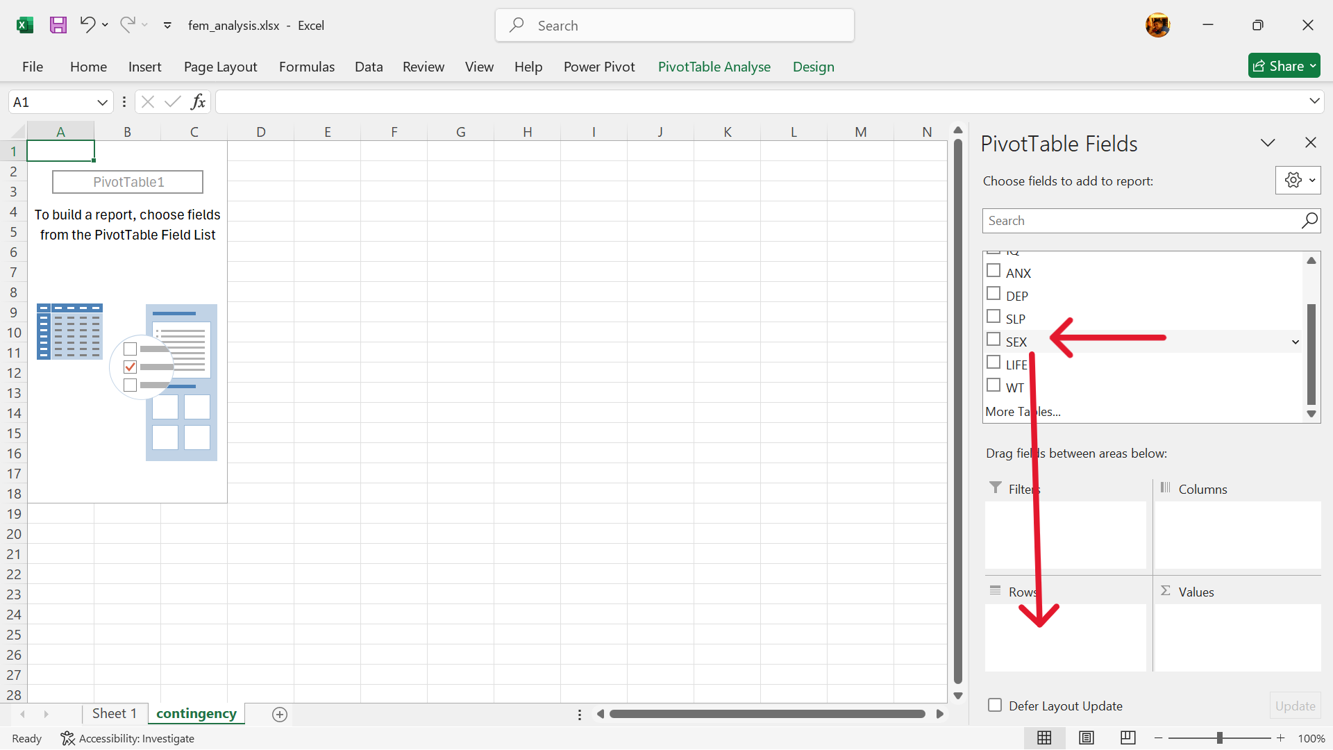
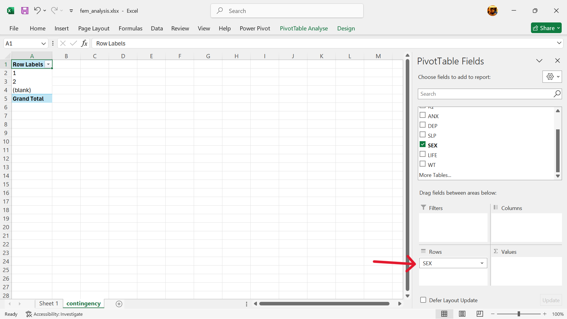
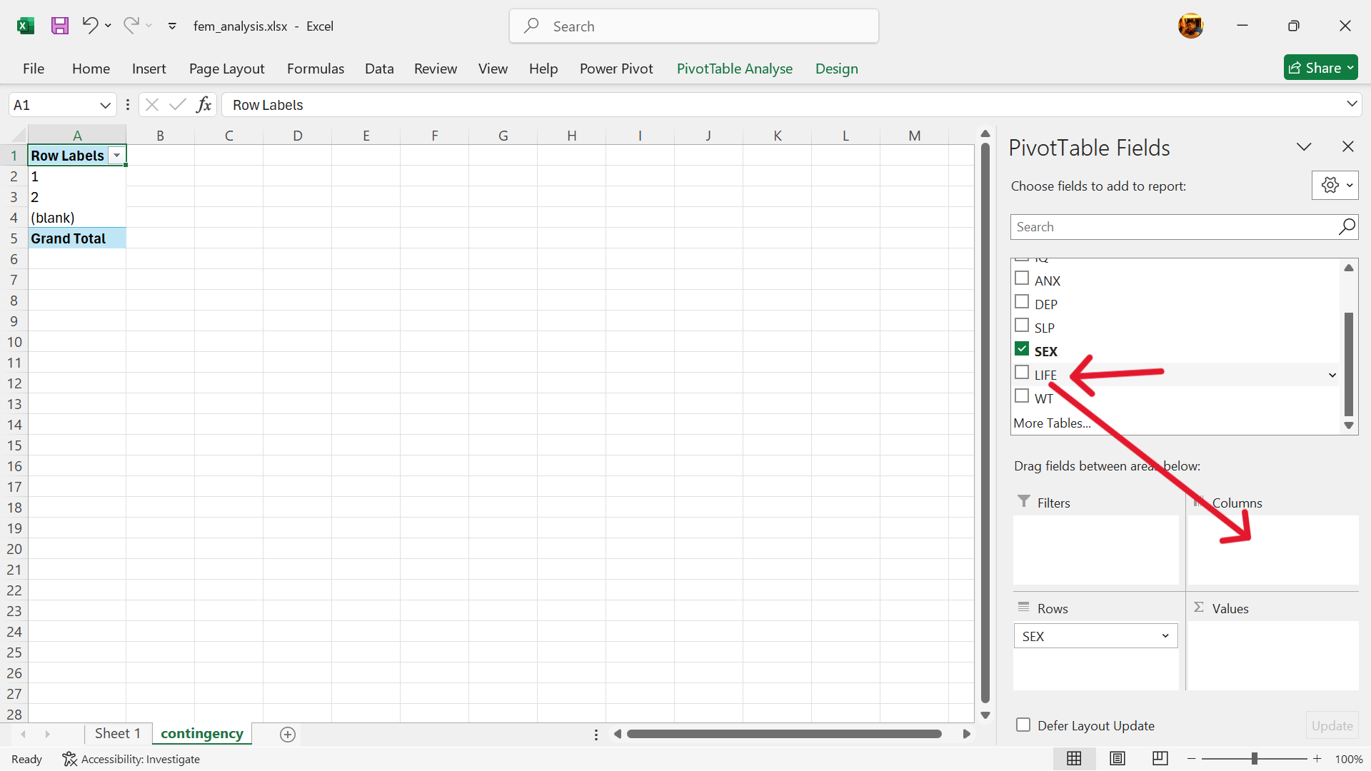
- Select exposure variable of contingency table.
The variable for no interest in sex (SEX) is the exposure variable. Select and drag to the rows setting.
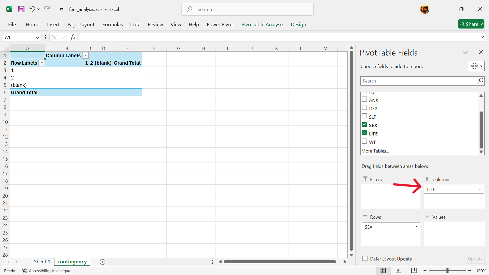
- Select outcome variable of contingency table.
The variable for considered suicide (LIFE) is the outcome variable. Select and drag to the columns setting.
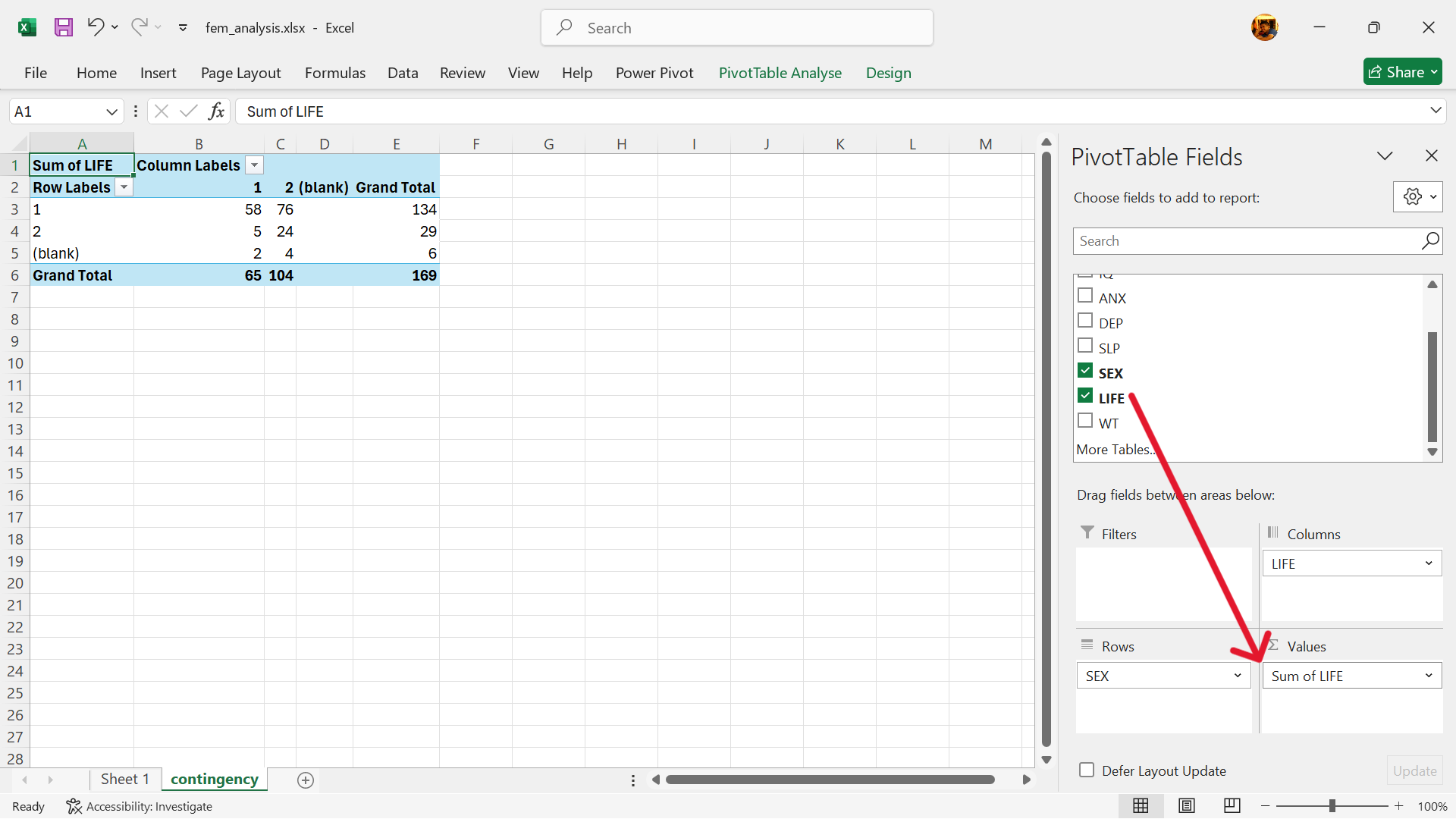
- Select values for the contingency table.
- Drag the
LIFEvariable into the values setting.
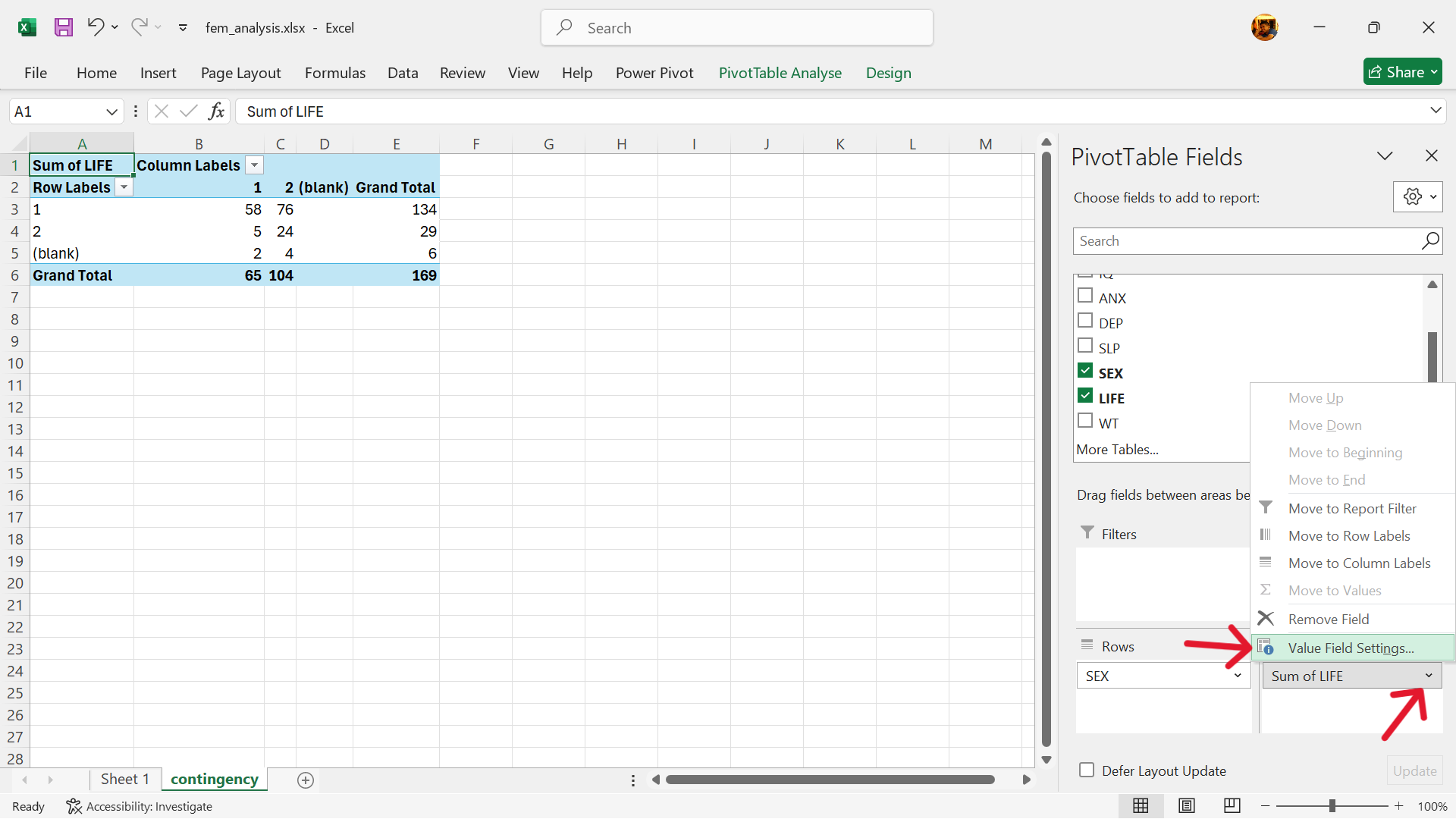
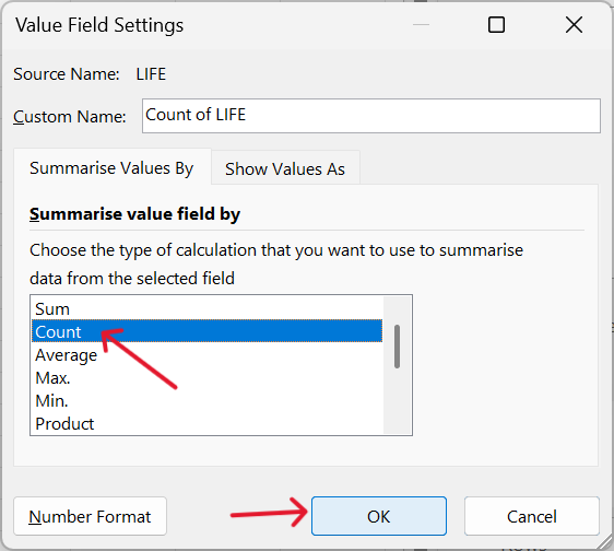
- Change the value setting to the COUNT summary measure.
Tap on the settings arrow on the value variable –> Value Edit Settings –> Select COUNT
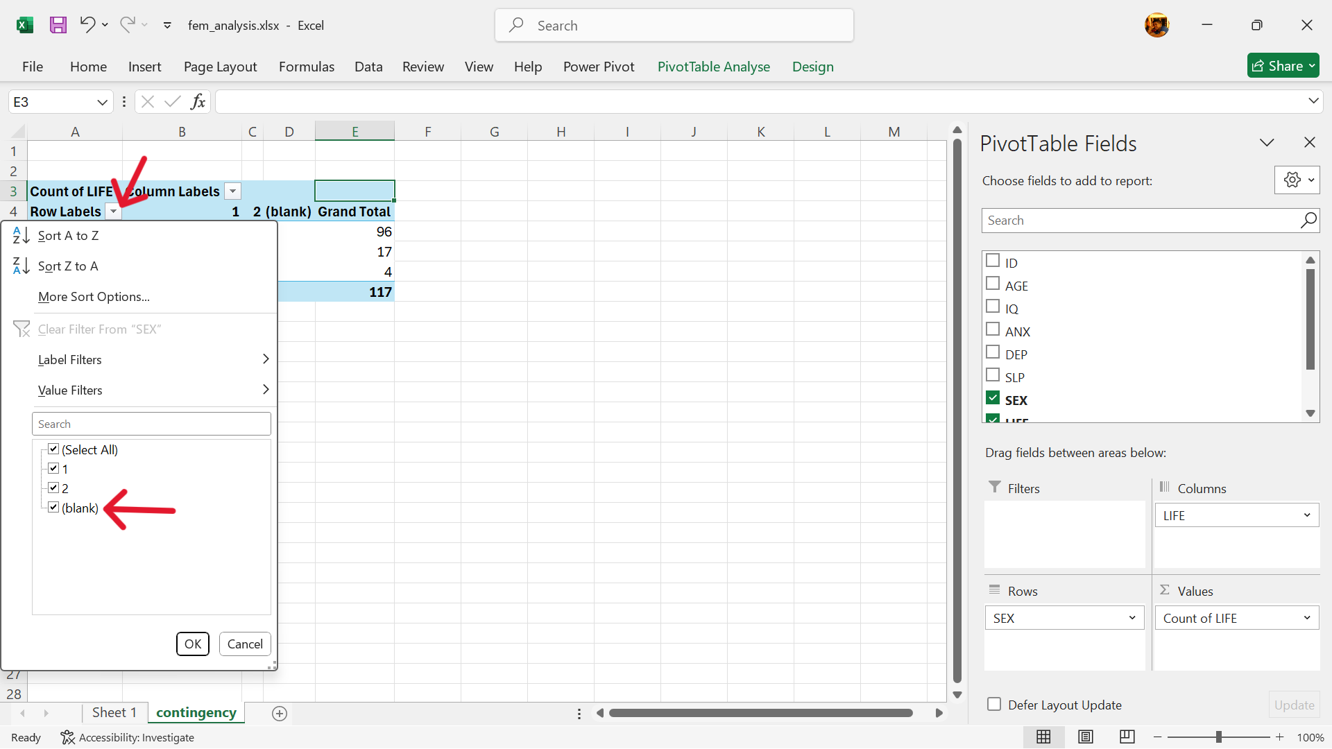
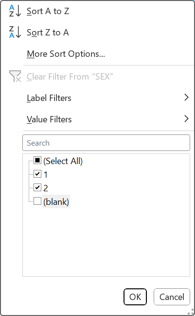
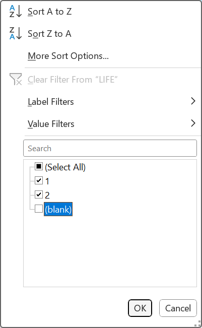
- Remove empty values in exposure variable.
- Click on settings button for exposure labels and untick blank.
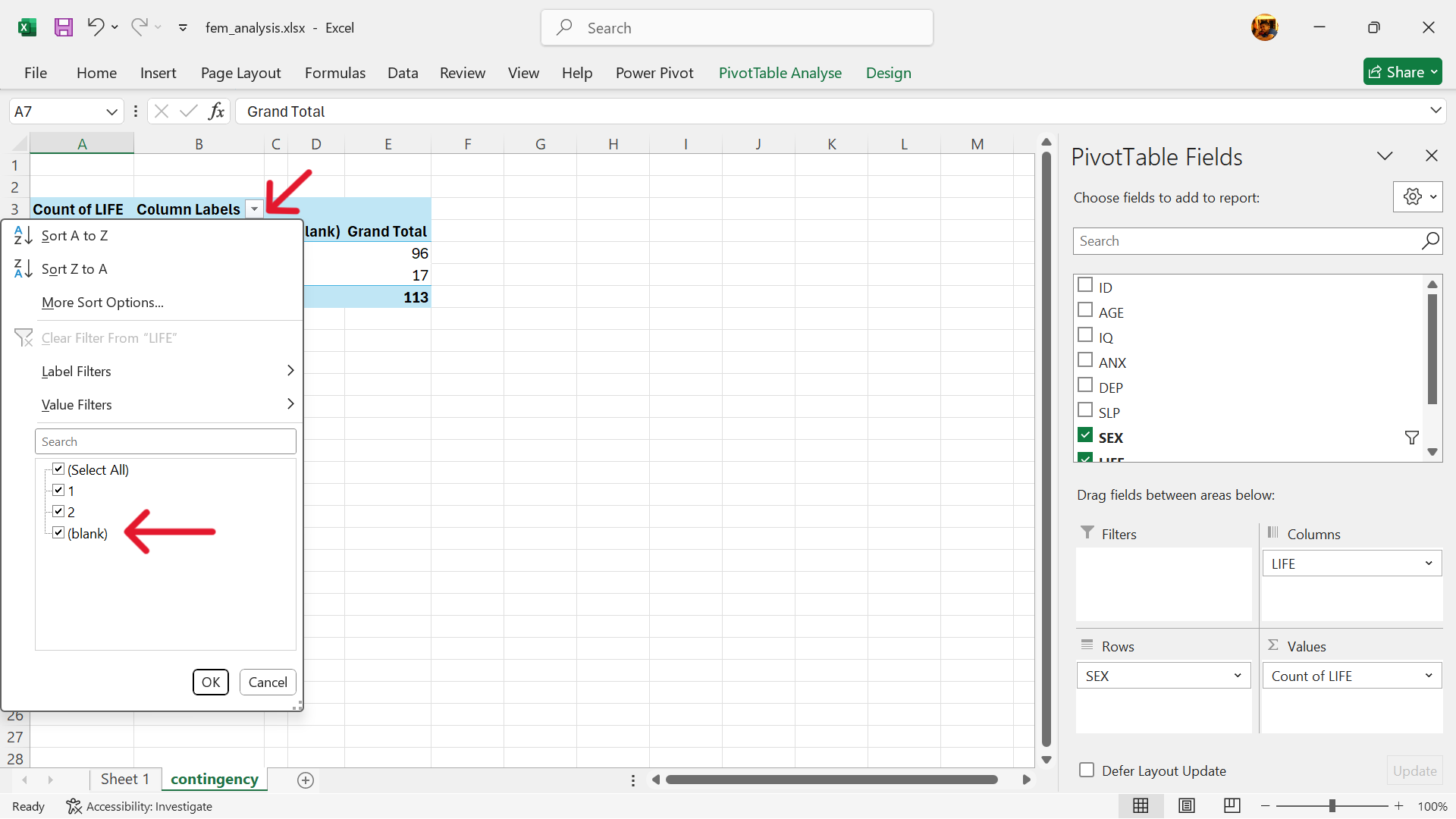
- Remove empty values in outcome variable.
- Click on settings button for outcome labels and untick blank.
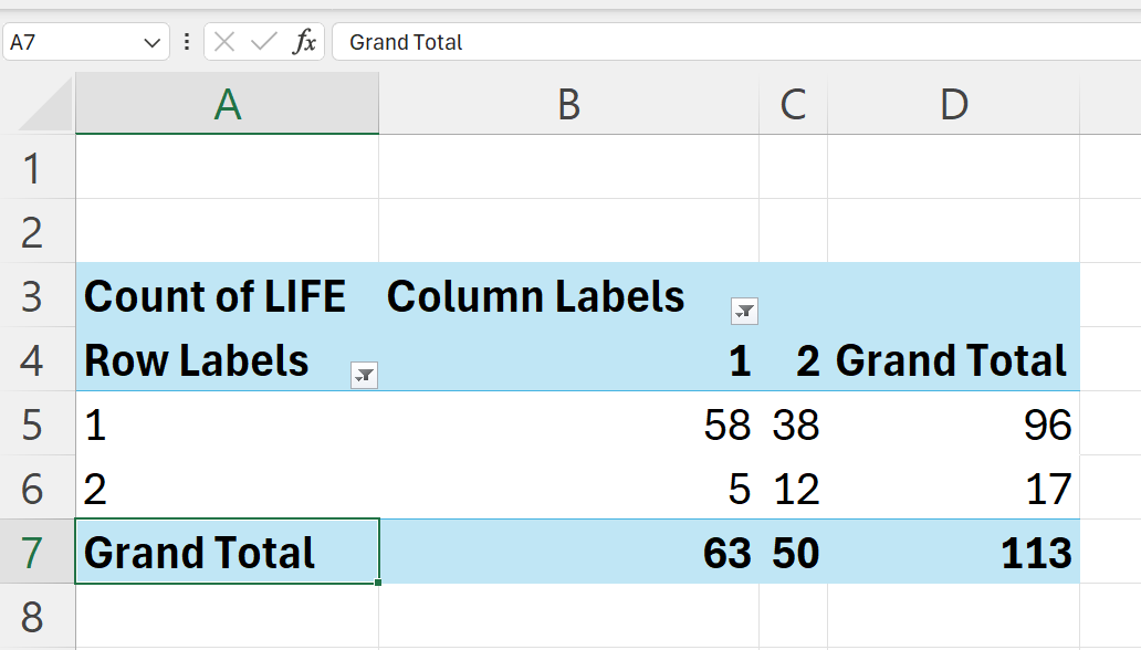
- Contingency table is now complete.
22.2 Relative risk ratio
Relative risk ratio (RRR) is a measure of the risk of a certain event happening in one group (usually called the exposed group) compared to the risk of the same event happening in another group (usually called the unexposed group). It indicates how much more likely the outcome is in the exposed group compared to the unexposed group.
22.2.1 Calculating relative risk ratio
Using the schema of a two-by-two table in Figure 22.1, the relative risk ratio is calculated as follows:
\[ RRR ~ = ~ \frac{\frac{A}{A + B}}{\frac{C}{C + D}} ~ = ~ \frac{A \times (C + D)}{C \times (A + B)} \]
where:
\(A ~ = ~ \text{exposed with outcome}\)
\(B ~ = ~ \text{exposed with no outcome}\)
\(C ~ = ~ \text{not exposed with outcome}\)
\(D ~ = ~ \text{not exposed with no outcome}\)
Using the pivot table we created in Section 22.1.1, we can calculate the relative risk ratio as follows:
\[ RRR ~ = ~ \frac{A \times (C + D)}{C \times (A + B)} \]
\[ RRR ~ = ~ \frac{58 \times (5 + 12)}{5 \times (58 + 38)} ~ = ~ \frac{58 \times 17}{5 \times 96} ~ = ~ \frac{986}{480} ~ = ~ 2.054167 \]
We can also perform this calculation in Excel using the pivot table we created.
=(B5*D6)/(B6*D5)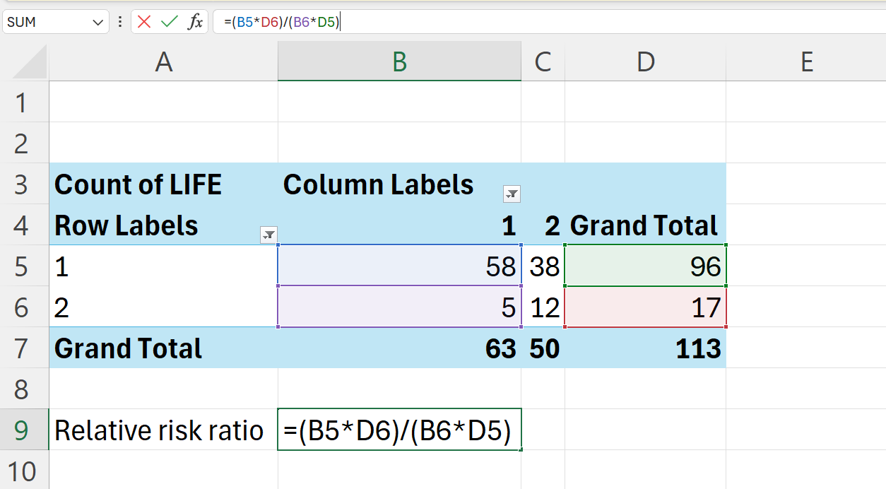
Calculating the confidence interval of the relative risk ratio
Following are the steps to calculating the confidence interval1 of the relative risk ratio.
- Calculate the standard error of the natural logarithm of relative risk ratio
\[ SE_{log(RRR)} ~ = ~ \sqrt{\frac{C}{A(A+C)} ~ + ~ \frac{D}{B(B+D)}} \]
In Excel, this can be calculated as follows:
=SQRT(B6/(B5*B7)+C6/(C5*C7))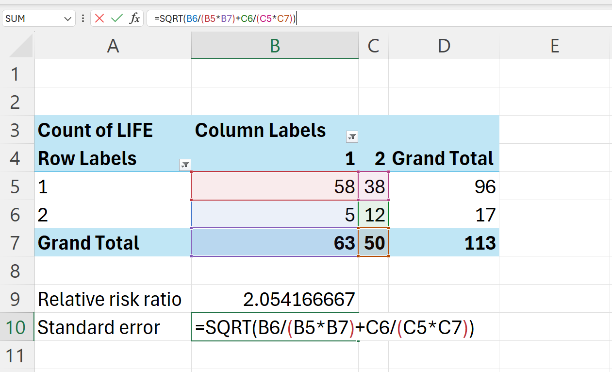
- Calculate the 95% confidence interval of relative risk ratio.
\[ 95\% ~ CI ~ = ~ e ^ {\log(RRR) ~ \pm ~ 1.96 ~ \times ~ SE_{\log(RRR)}} \]
In Excel, this can be calculated as follows:
=EXP(LN(B9)-1.96*B10) ## 95% LCI=EXP(LN(B9)+1.96*B10) ## 95% UCI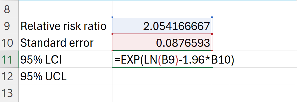
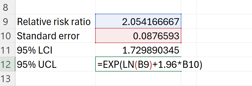
The risk of suicidal ideation for those with no interest in sex is 2.05 (95% CI: 1.7298903-2.4392302) times higher than those who have interest in sex.
22.2.2 Interpreting the relative risk ratio and its confidence interval
Table 22.1 provides guidance on how to interpret relative risk ratio.
| Risk ratio | Interpretation |
|---|---|
RRR = 1 |
Exposure does not affect outcome |
RRR < 1 |
Risk of outcome is decreased by the exposure (protective factor) |
RRR > 1 |
Risk of outcome is increased by the exposure (risk factor) |
If the 95% confidence interval doesn’t contain 1, this means that the risk of the outcome given the exposure is significant.
22.3 Odds ratio
Odds ratio (OR) is a measure of association between an exposure and an outcome. It represents the odds that an outcome will occur given a particular exposure compared to the odds of the outcome occurring in the absence of the exposure.
22.3.1 Calculating odds ratio
Using the schema of a two-by-two table in Figure 22.1, the odds ratio is calculated as follows:
\[ OR ~ = ~ \frac{A/B}{C/D} ~ = ~ \frac{A \times D}{B \times C} \]
\[ OR ~ = ~ \frac{58 \times 12}{38 \times 5} ~ = ~ \frac{696}{190} ~ = ~ 3.663158 \]
We can also perform this calculation in Excel using the pivot table we created.
=(B5*D6)/(B6*D5)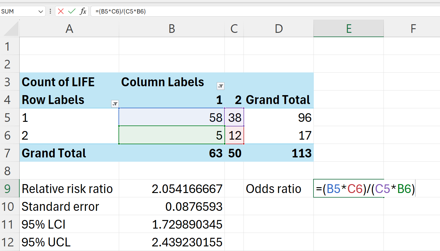
Calculating the confidence interval of the odds ratio
The 95% confidence interval is calculated as follows:
\[ 95\% ~ CI ~ = ~ e ^ {\log(OR) ~ \pm ~ 1.96 ~ \times ~ \sqrt{\frac{1}{A} + \frac{1}{B} + \frac{1}{C} + \frac{1}{D}}} \]
In Excel, this can be calculated as follows:
=EXP(LN(E9)-1.96*SQRT(1/B5+1/C5+1/B6+1/C6)) ## 95% LCI=EXP(LN(E9)+1.96*SQRT(1/B5+1/C5+1/B6+1/C6)) ## 95% UCI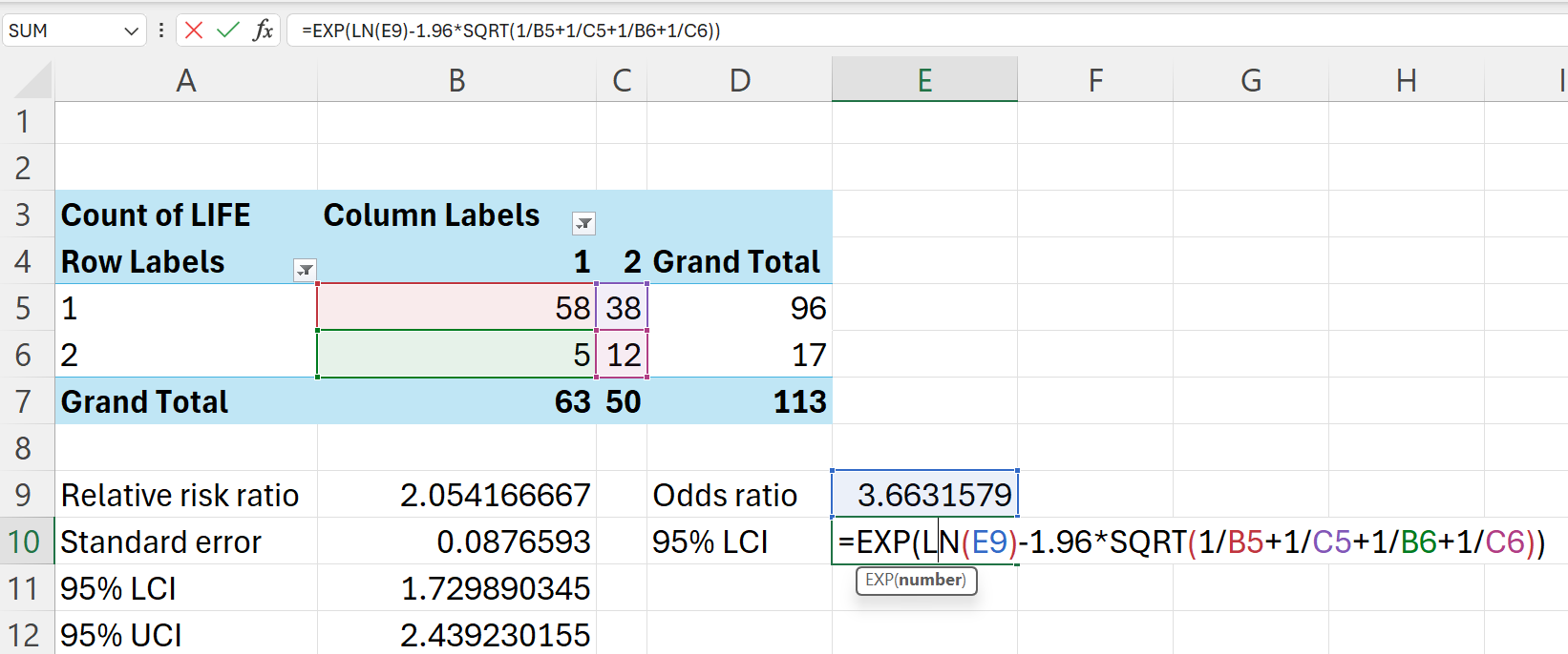
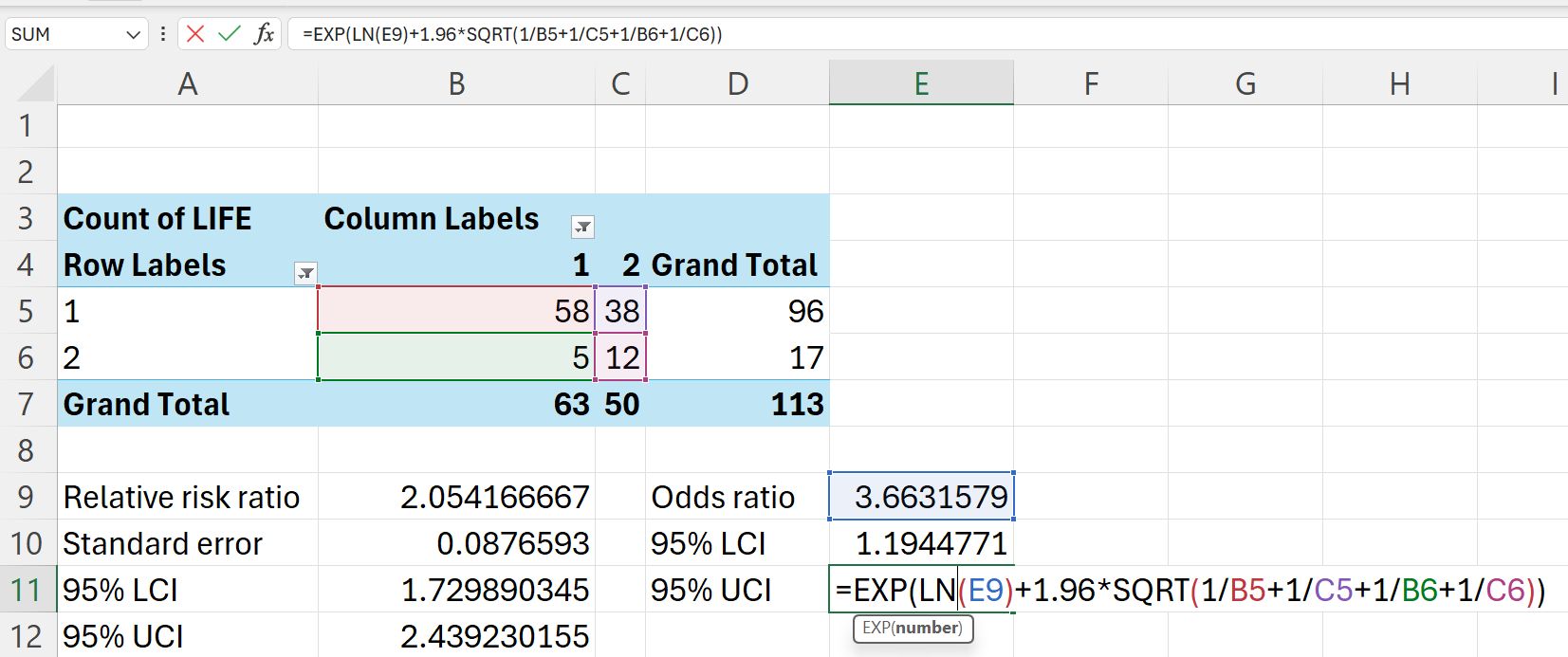
The odds of suicidal ideation for those with no interest in sex is 3.66 (95% CI: 11.2339746-2.4392302) times higher than those who have interest in sex.
22.3.2 Interpreting the odds ratio and its confidence interval
Table 22.2 provides guidance on how to interpret odds ratio.
| Odds ratio | Interpretation |
|---|---|
OR = 1 |
Exposure does not affect odds of outcome |
OR > 1 |
Exposure associated with higher odds of outcome |
OR < 1 |
Exposure associated with lower odds of outcome |
If the 95% confidence interval doesn’t contain 1, this means that the odds of the outcome given the exposure is significant.
22.4 Difference between relative risk ratio and odds ratio
Relative risk ratio approximates odds ratio for outcomes that are rare (< 10%) and as such can be reported interchangeably. In non-rare outcomes, odds ratio will tend to have greater magnitude than relative risk ratio but always in the same direction (negative or positive). In specific study designs, the total population-at-risk is not known hence relative risk ratio cannot be calculated.
22.5 Student t-test
Sometimes, we want to compare summary numerical values between one group and another. Unlike a contingency table that summarises the counts of the variables, this summary table will usually have the mean or median of the numerical values. We can use the t-test (also known as the Student t-test) to compare whether the mean of the values for one group is different from another group.
22.5.1 Calculating the t-test
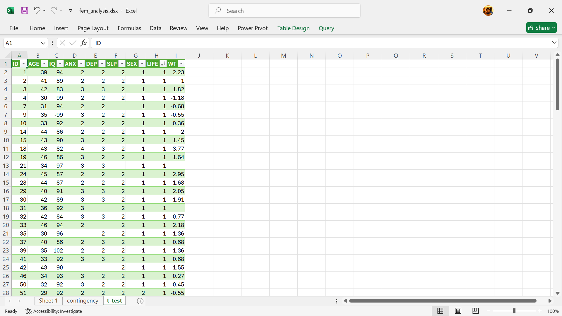
Using the fem dataset, let’s say for example we wanted to compare the mean age of those who have had thoughts of suicide to those who haven’t had thoughts of suicide. We can use the t-test to compare their mean age. In Excel, there is a built in function that performs the t-test, the T.TEST() function. Following are the steps on how to get the mean age for each group and then how to test if there is a difference between the mean age of the two groups.
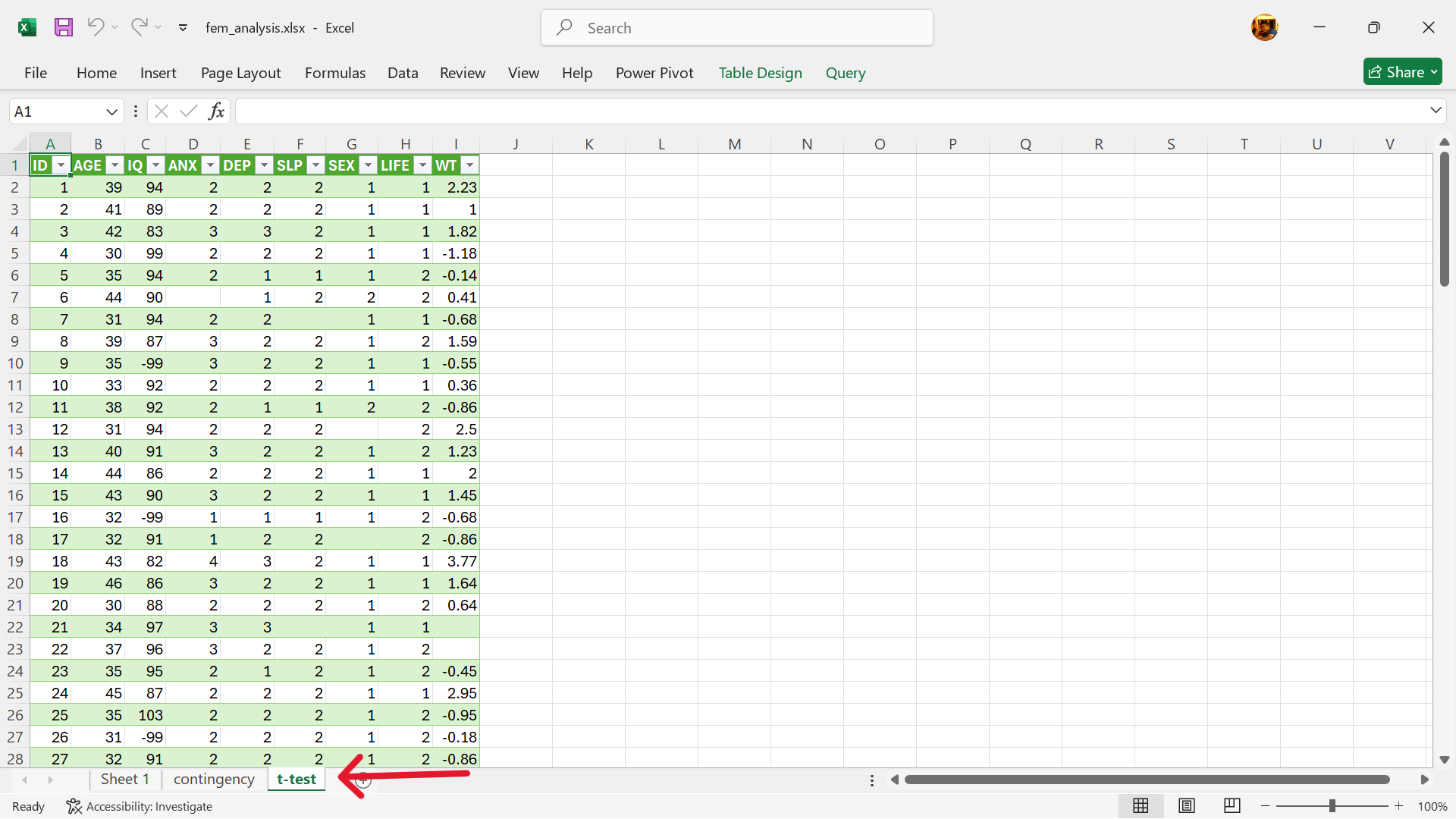
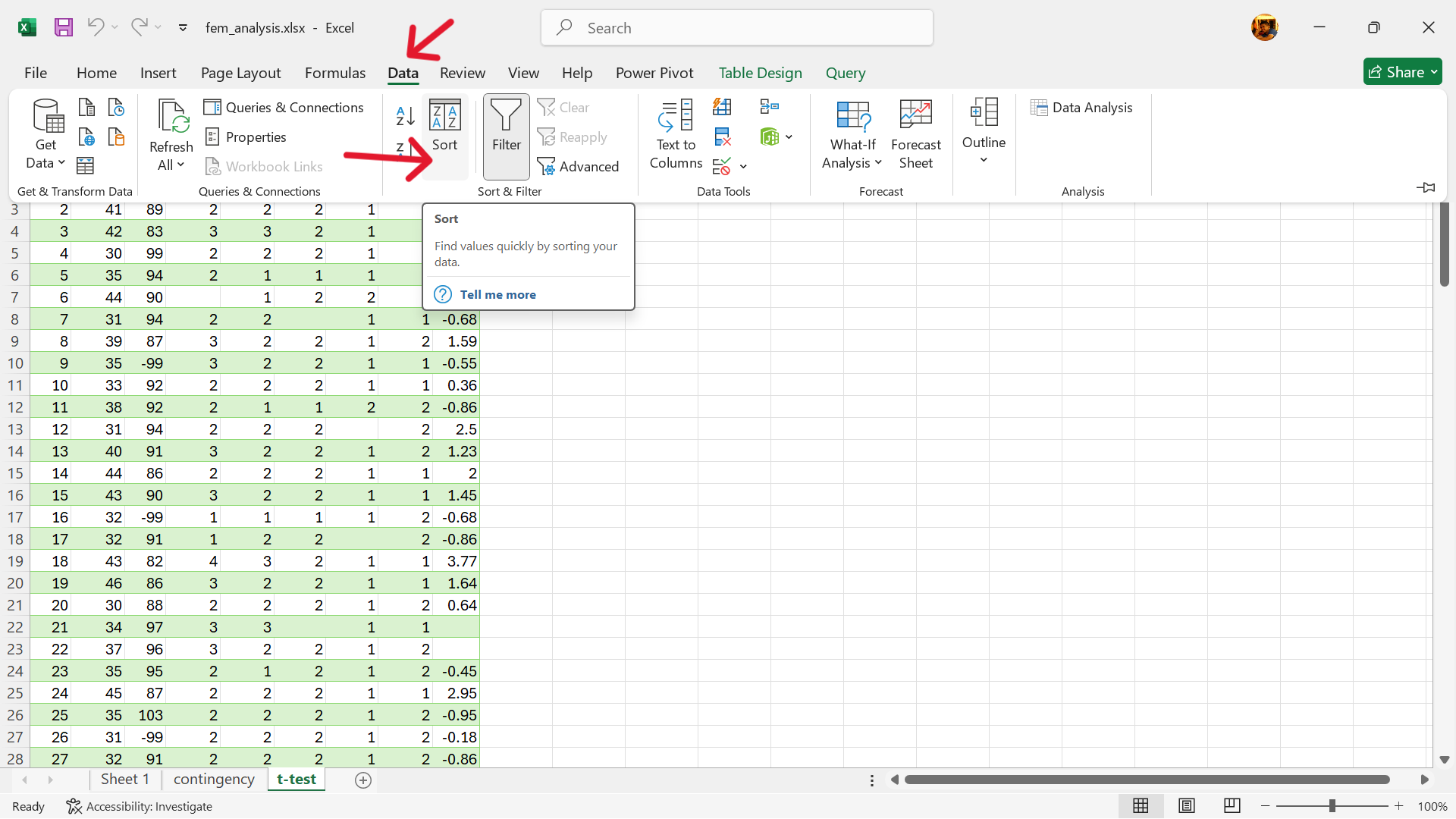
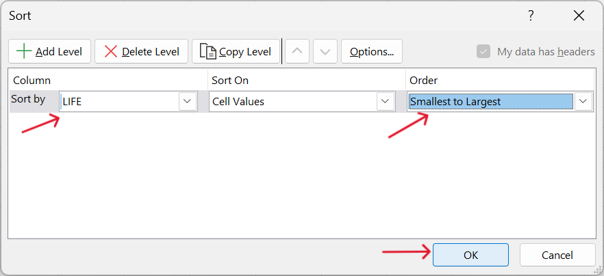
- Sort the fem dataset by the values of the
LIFEvariable.
We recommend doing this step on a new worksheet with a fresh instance of the fem dataset imported in (Figure 22.26). Then sort the whole table based on the values of the LIFE variable (Figure 22.27).
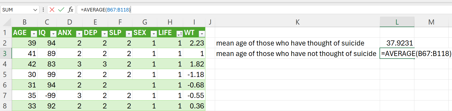
- Get the mean age for the each group value of
LIFEvariable.
=AVERAGE(B2:B66) ## Average age of those who thought of suicide=AVERAGE(B67:B118) ## Average age of those who have not thought of suicide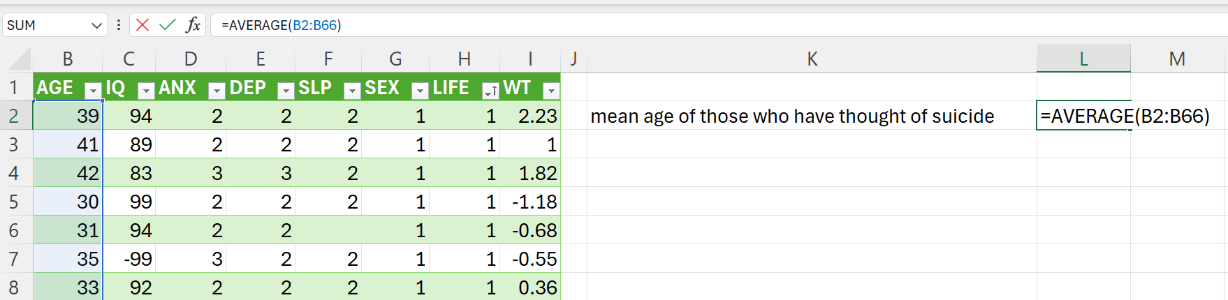
- Perform t-test on
AGEvariable between the two groups.
Using the T.TEST() function:
=T.TEST(B2:B66,B67:B118,2,2)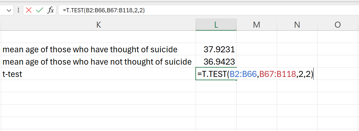
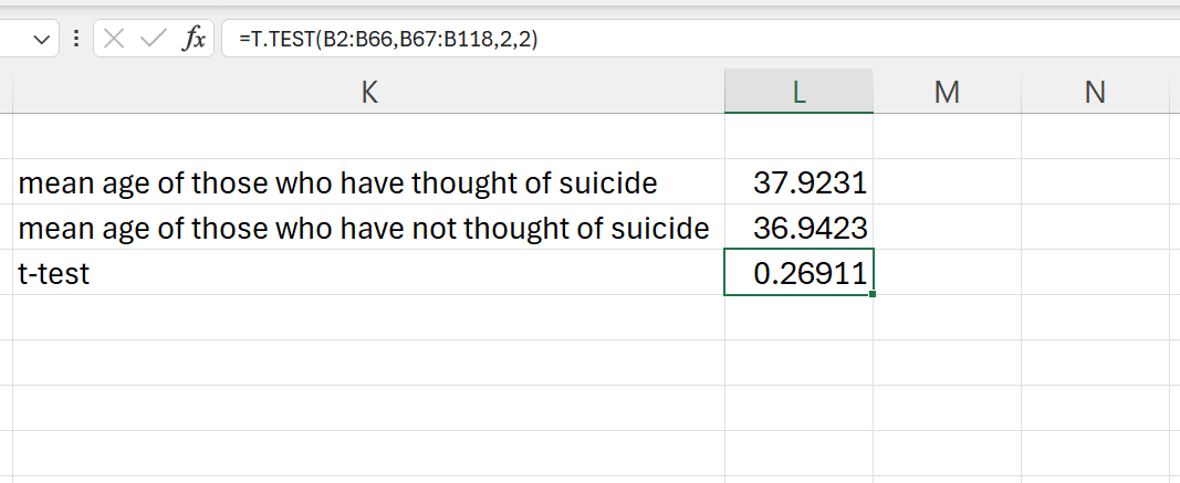
The result of the t-test is the p-value for the test. The result is 0.2691091. These is no significant difference between the mean ages of those who thought of suicide and to those who had no thoughts of suicide.
A confidence interval is a specific range of values, determined using sample data, which probably includes the actual value of an unknown population parameter. It shows how much uncertainty about a sample statistic and provides a likely interval for the corresponding population parameter. For instance, a 95% confidence interval means that if we repeated the sampling and calculation process numerous times, 95% of those intervals would include the true population parameter.↩︎